Sparse Matrices

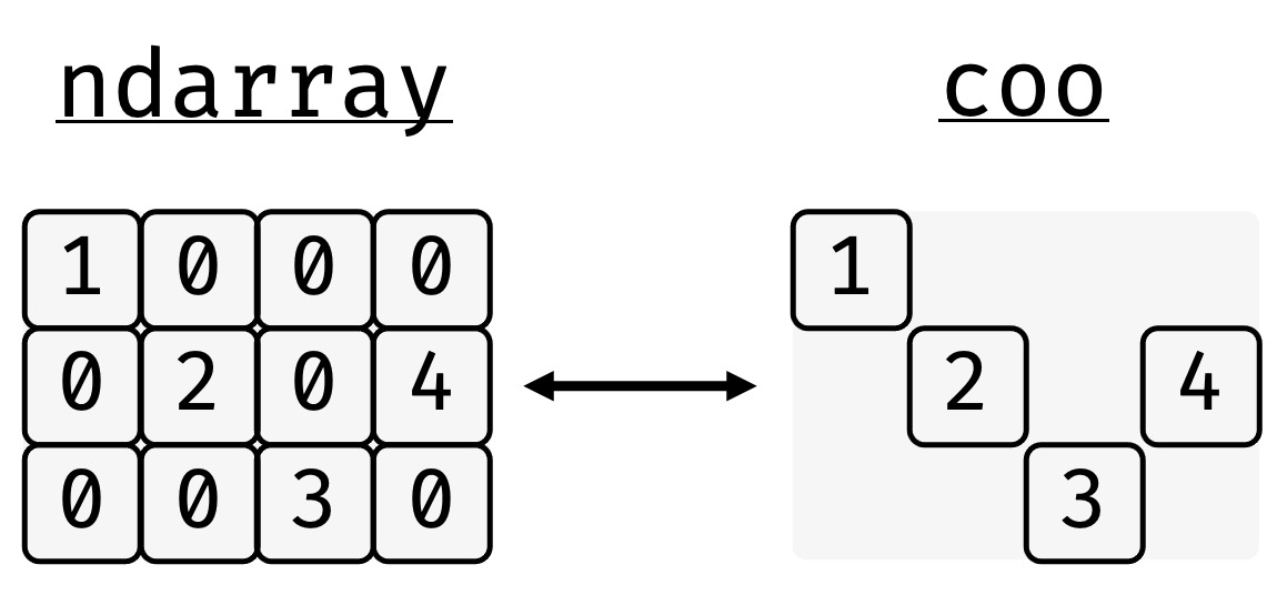
A sparse matrix is a matrix, which contains mostly zeros. Rather than storing the zeros explicitly, only the non-zero values are stored together with information that allows one to reconstruct the equivalent dense matrix.

>>> import bsparse.sparse as sp
>>> import numpy as np
>>> arr = np.array(
...     [
...         [1, 0, 0, 0],
...         [0, 2, 0, 4],
...         [0, 0, 3, 0],
...     ]
... )

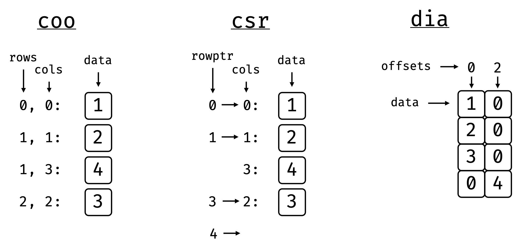
The equivalent dense matrix can be stored in different equivalent ways. In bsparse the coordinate (COO), compressed sparse row (CSR), and the diagonal (DIA) storage schemes are implemented.

bsparse facilitates the conversion between these storage formats as well as their creation from sparrays or ndarrays.

>>> coo = sp.COO.from_array(arr)
>>> coo
COO(shape=(3, 4), nnz=4, dtype=int64)
>>> coo.tocsr()
CSR(shape=(3, 4), nnz=4, dtype=int64)
>>> coo.todia()
DIA(shape=(3, 4), nnz=8, dtype=int64)

All sparse matrices have a datatype of the underlying scalars (.dtype), a 2D matrix shape (.shape), a number of explicitly stored values (.nnz), and a symmetry attribute (.symmetry).

>>> coo.dtype
dtype('int64')
>>> coo.shape
(3, 4)
>>> coo.nnz
5
>>> coo.symmetry  # None

The matrix can be sliced and elements can be set and accessed using NumPy-style indexing.

>>> coo[1, 1]
2
>>> coo[2, 3] = 5
>>> coo[2, 3]
5
>>> coo[:2, 1::2]
COO(shape=(2, 2), nnz=2, dtype=int64)
>>> coo[:2,1::2].toarray()
array([[0, 0], [2, 4]])

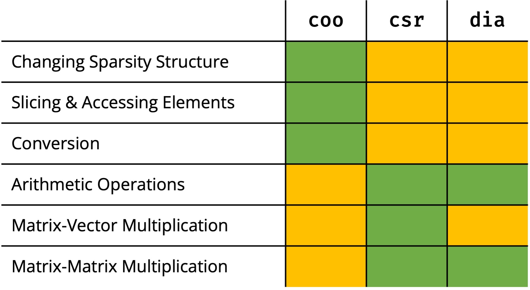
Sparse matrices also support mathematical operations, which – depending on the storage scheme – can differ in efficiency. Here an overview to give you a very rough rule of thumb (DYOB – do your own benchmarking!)